1.识别系统简介
在文字识别系统中,通常包括CNN进行提取特征;一个RNN进行序列化消息传递;最后一个CTC loss 来作为目标函数优化
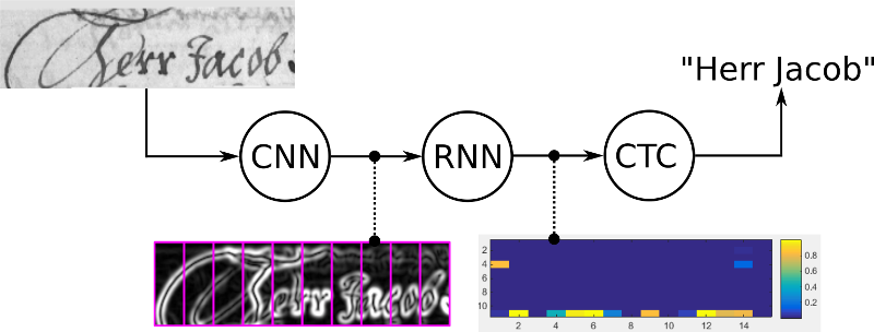
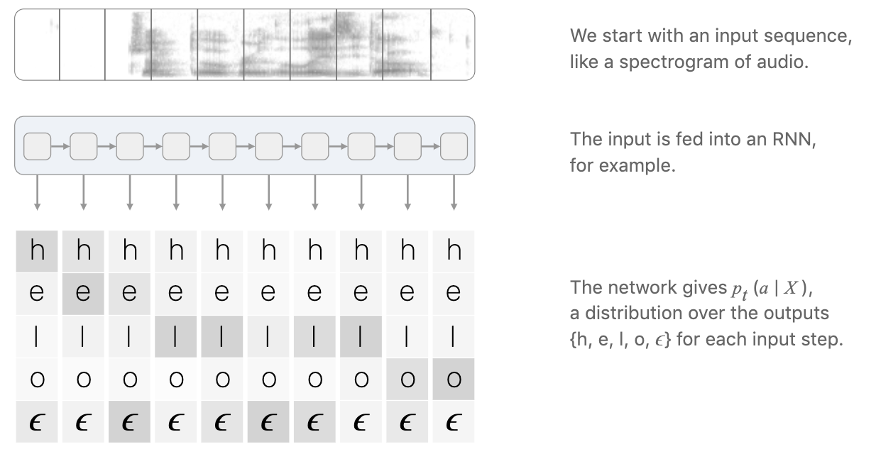
RNN输出character-score的分数矩阵。如下,在各个时刻分别是各个字符的概率,颜色越深,概率越大:
得到这个分数矩阵之后,?首先需要考虑下面两个问题:
- 我们要怎么建立目标方程来训练这个网络呢?
- 如何根据这个分数矩阵得到结果呢?
2.Naive方法:使用传统监督方法
输入的序列(即序列化模型的输出结果,如RNN)为:$X=[x_1,x_2,…,x_T]$ 预测的文本序列为:$Y=[y_1,y_2,…,y_U]$
我们需要找到一个从$X$到$Y$的映射,用传统的监督学习方法,我们需要标注每个字符,然后和ground truth进行alignment,再对每个识别的字符算loss。这种方法的问题是:
- character-level的标注不现实
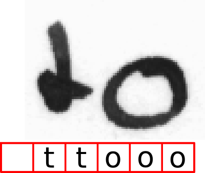
- 我们只得到了字符的分数,需要额外的处理来得到最后的文本内容,比如得到“ttooo”,但是它实际上可能是“to”或者“too”.
3.CTC方法
从上面的描述,我们知道基于character-level的标注方法是不可行的,但是不进行character-level的标注,又不知道怎么进行alignment。因此这里借用语音 识别系统中的CTC 方法。字符识别这个问题和语音识别具有很大的相似性,都是根据序列化信息来预测文本输出。而CTC 方法的优点是:
- 不需要character-level的标注,我们不关注每个字符的宽度或者位置
- 不需要额外的识别文字。
4.CTC的原理
4.1Alignment
为了给定的输入$X$和输出$Y$计算loss,CTC将所有可能对齐的方式进行loss加和。
it tries all possible alignments of the GT text in the image and takes the sum of all scores. This way, the score of a GT text is high if the sum over the alignment-scores has a high value.
举个例子,下面的$X$,在和label进行alignment的时候是很不好做的,首先,将X里面的每个字符和Y的字符进行对齐是不科学的,因为字符之间有时候存在很大间隙;另外,没有办法产生带有重复字符的text,比如“hello”和“helo”。
 为了区分重复字符(如“helo”和“hello”)以及解决字符之间存在一些间歇等问题,我们引入伪字符 blank token:$\epsilon$。
The ϵ token doesn’t correspond to anything and is simply removed from the output.
这个$\epsilon$的放置要求就是在重复字符之间,一定至少要有一个。比如下面的这几种放置方法,如果目标是“cat”,那么前三种方法是对的,后三种方法是错的,因为后面三种经过 去重、移除$\epsilon$ 之后是不能得到目标“cat”的;在计算loss的时候,我们就会将能转换成目标“cat”的所有可能的alignments计算loss再加和,也就是说CTC的alignment是many-to-one的:

为了更好理解,再举个例子,对于“hello”这个目标,根据RNN,有可能会得到下面这样的输出,并拿出其中有可能的三个alignments进行去重,移除$\epsilon$等操作,得到了三个结果(倒数第二行和倒数第三行应该是反了):

4.2损失函数
根据上面的分析,我们就知道怎么计算损失函数了,对于一对$(X,Y)$,我们建立下面的条件概率:
| 由于每个alignment都是由$T$个time step输出的字符组成的,那么每个time step输出的字符都有一个概率$p_t(a_{t} | X)$.$P(Y | X)$就是给定RNN 的输出$X$,我们能经过去重、移除操作后得到$Y$的概率。为了代替最大似然估计,我们用最小化负对数损失来代替,对于N个样本${(X_1,Y_1),(X_2,Y_2),…,(X_N,Y_N)}$,那么损失函数就是: |
\begin{equation} L=\sum ^{N}_{i=1}( -log( P( Y_{i} |X_{i})) \end{equation}
举个例子:
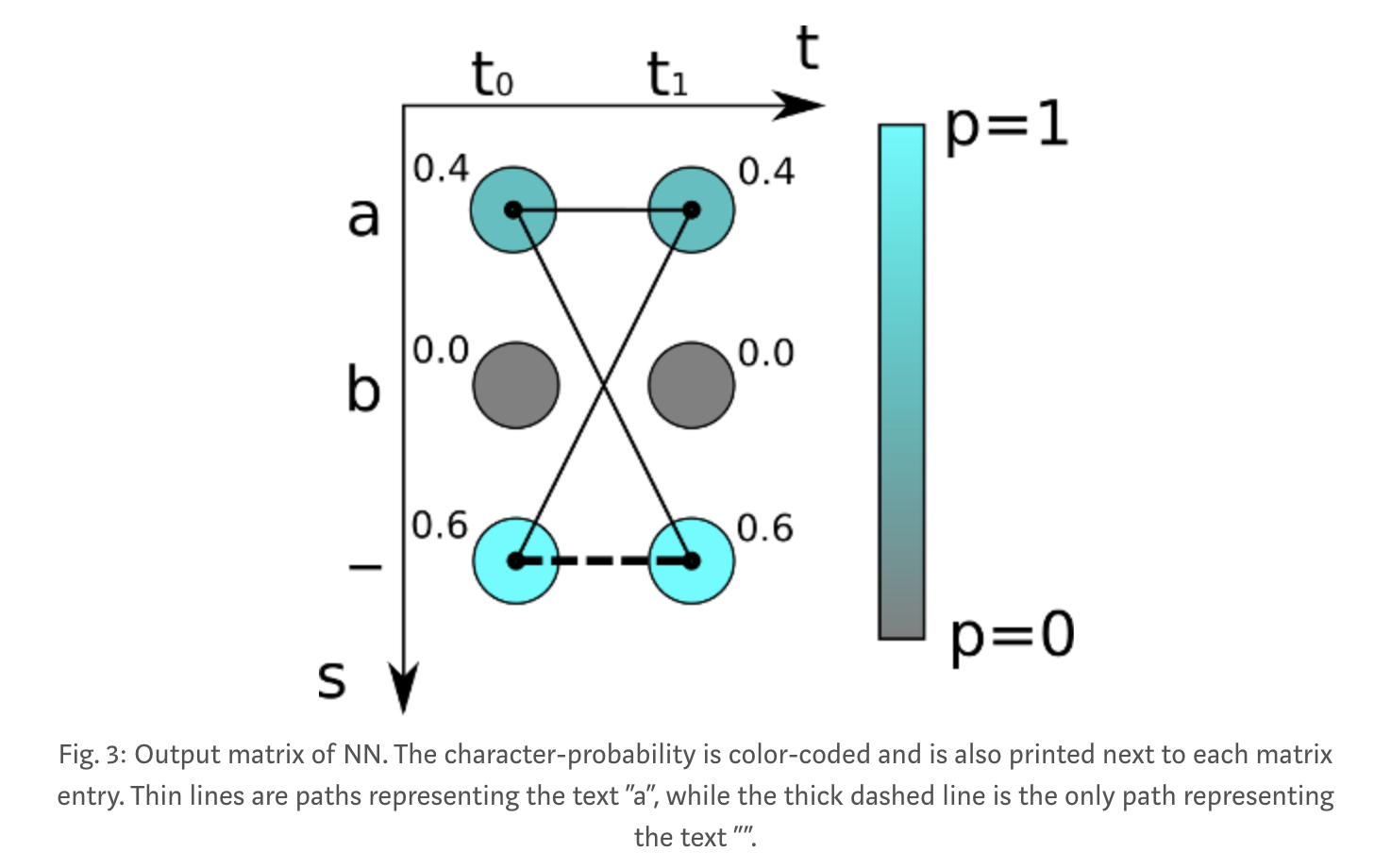
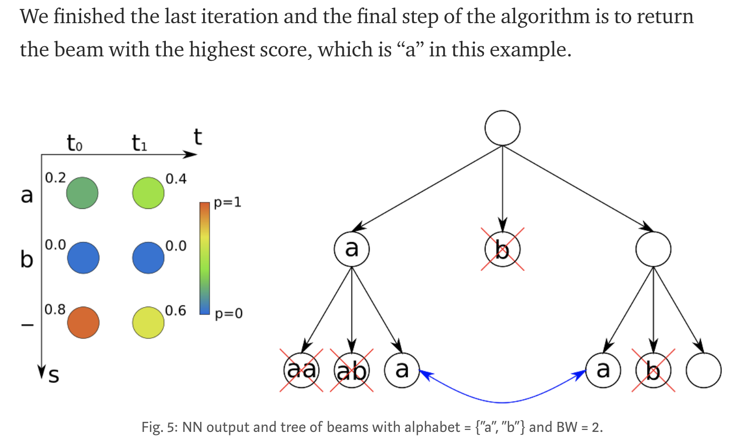
The score for one alignment (or path, as it is often called in the literature) is calculated by multiplying the corresponding character scores together. In the example shown above, the score for the path “aa” is 0.4·0.4=0.16 while it is 0.4·0.6=0.24 for “a-” and 0.6·0.4=0.24 for “-a”. To get the score for a given GT text, we sum over the scores of all paths corresponding to this text. Let’s assume the GT text is “a” in the example: we have to calculate all possible paths of length 2 (because the matrix has 2 time-steps), which are: “aa”, “a-” and “-a”. We already calculated the scores for these paths, so we just have to sum over them and get 0.4·0.4+0.4·0.6+0.6·0.4=0.64. If the GT text is assumed to be “”, we see that there is only one corresponding path, namely “–”, which yields the overall score of 0.6·0.6=0.36.you have seen that we calculated the probability of a GT text, but not the loss. However, the loss simply is the negative logarithm of the probability.
4.3损失的计算-动态规划
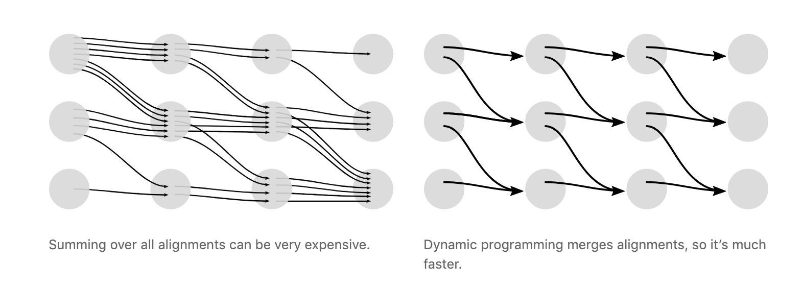
CTC loss有一个问题就是计算量非常庞大,因为所有可能的alignments数量是很多的,速度回很慢,因此使用动态规划的方法来计算loss,它的思想就是:
if two alignments have reached the same output at the same step, then we can merge them
解决方法(不是很懂)
假设$T$个time step的序列分数我们表示成:
\begin{equation} Z=[ \epsilon ,y_{1} ,\epsilon ,y_{2} ,…,\epsilon ,y_{U} ,\epsilon ] \end{equation}
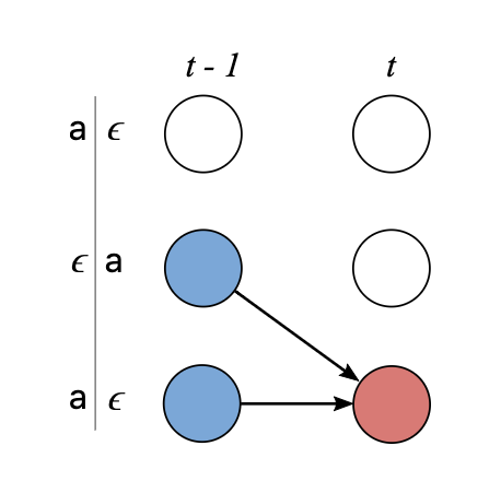
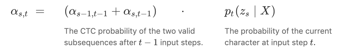
假设$\alpha_{s,t}$是合并后的某个节点的分数,也就是子序列$Z_{1:s}$在t时刻的分数.我们计算$\alpha_{s,t}$时存在两种情况:
-
我们不能跳离上一个字符,首先因为上一个字符可能是标签中的一个字符,那么此时$Z_s=\epsilon$;其次,在重复的字符之间必须有一个$\epsilon$,即$Z_s=Z_{s-2}$.因此有下面的递推式:
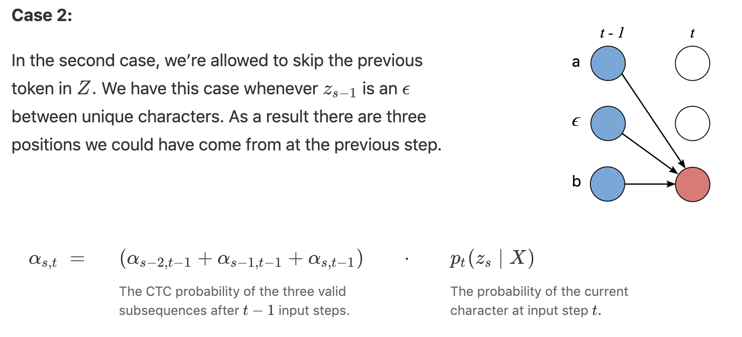
-
能跳离上一个字符
5.Inference(测试)
在测试时就没有标签了,我们没办法得到想要的alignments,只能用其他的方法来做,下面讲2种方法。
5.1 best path decoding
是一种启发式算法,就是在每一个time step都选择最大概率的字符,然后再经过去重和移除blank,如下选择虚线链接的路径。
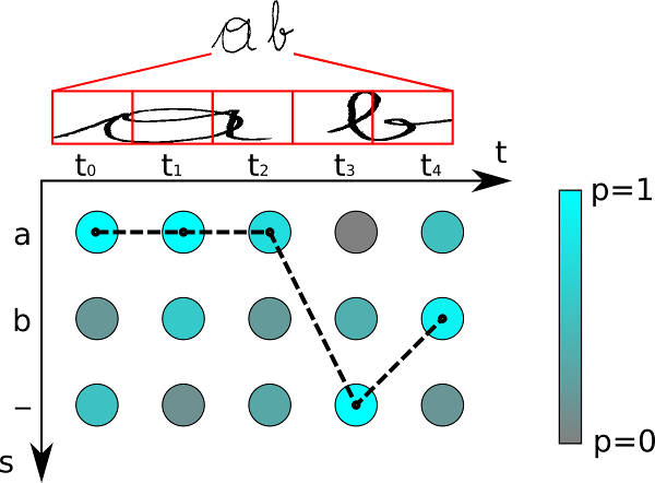
但是它的问题就是没考虑所有的alignments,也就是“多对一”问题,虽然单个路径可能分数很高,但是多对一的alignments加起来分数会更高。
Here’s an example. Assume the alignments [a, a, \epsilonϵ] and [a, a, a] individually have lower probability than [b, b, b]. But the sum of their probabilities is actually greater than that of [b, b, b]. The naive heuristic will incorrectly propose Y =Y= [b] as the most likely hypothesis. It should have chosen Y =Y= [a]. To fix this, the algorithm needs to account for the fact that [a, a, a] and [a, a, \epsilonϵ] collapse to the same output.
5.2 beam-search decoding[参考3、4]
5.2.1 基本版本
Beam search decoding iteratively creates text candidates (beams) and scores them.
伪代码如下:
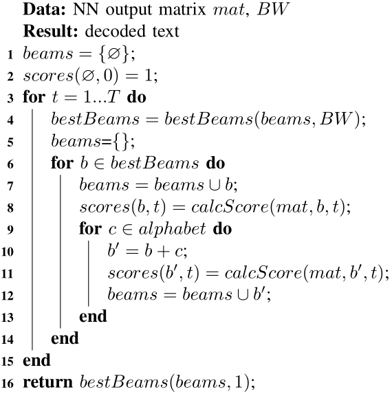
(1)the list of beams is initialized with an empty beam (line 1) and a corresponding score (2). Then, the algorithm iterates over all time-steps of the NN output matrix (3–15). At each time-step, only the best scoring beams from the previous time-step are kept (4). The beam width (BW) specifies the number of beams to keep. For each of these beams, the score at the current time-step is calculated (8). Further, each beam is extended by all possible characters from the alphabet (10) and again, a score is calculated (11). After the last time-step, the best beam is returned as a result (16).
例子
5.2.2 改进版本:beam search+language module
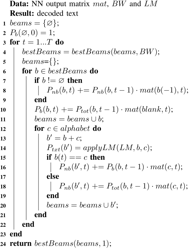
It is similar to the already shown basic version, but includes code to score the beams: copied beams (lines 7–10) and extended beams are scored (15–19). Further, the LM is applied when extending a beam b by a character c (line 14). In case of a single-character beam, we apply the unigram score P(c), while for longer beams, we apply the bigram score P(b[-1], c). The LM score for a beam b is put into the variable Ptxt(b). When the algorithm looks for the best scoring beams, it sorts them according to Ptot·Ptxt (line 4) and then takes the BW best ones.
时间复杂度
The running time can be derived from the pseudo code: the outer-most loop has T iterations. In each iteration, the N beams are sorted, which accounts for N·log(N). The BW best beams are selected and each of them is extended by C characters. Therefore we have N=BW·C beams and the overall running time is O(T·BW·C·log(BW·C)).
其他方法:prefix-search decoding or token passing
6.CTC in contexts
- HMMs
At a first glance, a Hidden Markov Model (HMM) seems quite different from CTC. But, the two algorithms are actually quite similar. Understanding the relationship between them will help us understand what advantages CTC has over HMM sequence models and give us insight into how CTC could be changed for various use cases.
- Encoder-Decoder models
We can interpret CTC in the encoder-decoder framework. This is helpful to understand the developments in encoder-decoder models that are applicable to CTC and to develop a common language for the properties of these models
7.参考文献
博客: 2.An Intuitive Explanation of Connectionist Temporal Classification